Johannes Lampel - Projects/SPCC

This project was motivated by an article on gamasutra : Image Compression with Vector Quantization by Ivan-Assen Ivanov.
And I already had a fine implementation of a SOM ( self organizing map ) simulator, therefore I tested if this wouldn't also work using LVQ ( linear vector quantization ), but also SOM. ( chapter about SOMs in german text about JoeBOT : chapter )

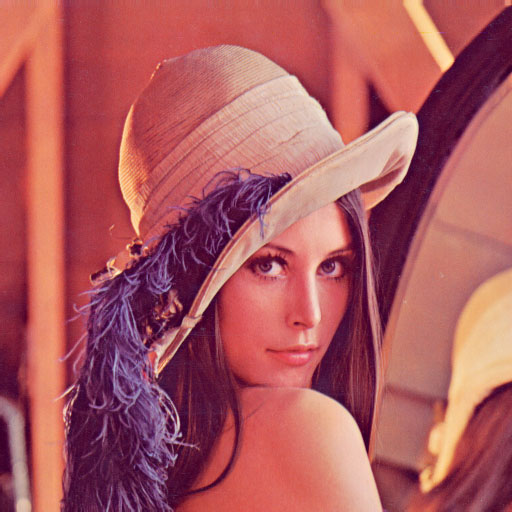
The example used here will be the lena picture, a picture used everywhere in texts about image compression. For more information about the background of this picture : http://www.lenna.org

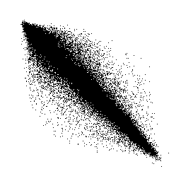
The rough idea of the system is that neighbouring pixels on a picture are usually in some way similar, and often structures are repeated, thus could be compressed. Imagine a greyscale picture and now look at neighbouring pixel pairs and draw them on a plane. Because in most cases, the greyscale values of both pixels are nearly the same, you'll fine most entries on the diagonal of that plane. This looks like this when you set a black dot for each existing pair :

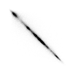
When looking at a density plot, you see that almost all pairs are on the diagonal :

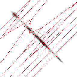
Now you want to describe those pairs, but with only a limited number of states, e.g. 16. You could just lay 16 squares over that area and then look in which of those square you can find such a pair of pixels, but the result would be pretty bad since you'd have some squares ( those on the diagonal ) with almost all pixelpairs in them and some away from the diagonal with just a few of them.

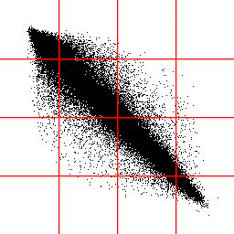
The solution herefore would be to use flexible areas, thus we'd have approximately the same amount of pixelpairs in each of them. The red dots are practically the 'center of mass' for each of those sectors, later called codebookvectors.
You can imagine the SOM as an elastic net wanting to approximate the density of the given data, thus minimizing the sum over the distances from each data entry to the next neuron on the SOM, the next codebookvectors - which are the red dots here.

The compression works as follows : First we store the grey values of the codebookvectors. Then we take each pixelpair of the original picture and search the nearest codebookvector and store its index. Because we only have 16 codebookvectors, we only need 4 bits for storing them. Storing the original grey values of 2 pixel would cost 16 bit.

Compressing colour pictures using this method is no problem, because the SOM algorithm works on any data we have a distance function for. When we only look at one pixel at a time and then use the algorithm we get some sort of indexed colours, i.e. we pick the most probable colours in the picture, store them and then only describe each pixel by telling the index of the colour from a colour table. This situation can still be visualized :

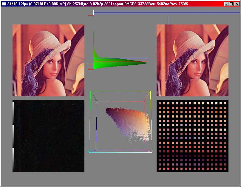
Here we see the original on the topleft corner, the compressed image on the topright, a normalized difference picture bottomleft and the codebookvectors bottomright. In the middle on top we can see the error distribution, i.e. how many pixels have a certain error, i.e. a certain distance to the next codebookvector. In the middle on the bottom we have a cube where the points are drawn at a location given by their color, in this case their red, green and blue parts are interpreted as a position in that cube. (0,0,0) would be in the black corner, (255,255,255) in the white corner. Normalized difference picture means that the difference is calculated and then we search the maximum and scale the whole picture so we have one pixel with a component of 255. The black-to-white bar on the left was before normalizing only once there, now one can see by how often the bar is show, how much the difference has been amplified for this picture.
In this case we used a SOM which was linear, not like that grid above at the greyscale pictures. Neighbouring codebookvectors in the SOM are connected by lines.

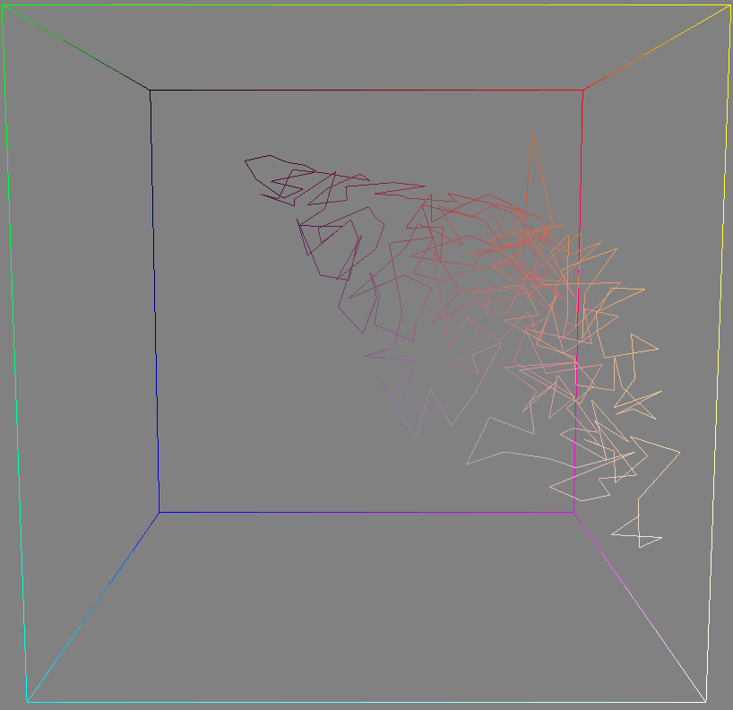
Using a square SOM, this looks similar, but you can see at the codebookvector picture bottomright the reason for the comparision of the SOM with an elastic net better : similar codebookvectors are close to each other.

If a square SOM or a linear one fits better depends on the distribution of the vectors the SOM is trained with. Often a linear SOM is better, but a linear SOM takes more time to train, because the distance factor is quite big in the beginning, since at first we need initialize all codebookvectors near to the average of our input data and then allowing it to specify on certain features by lowering the distance factor during training. Interestingly the colours inside this RGB color cube of most pictures are somewhat located on planes.

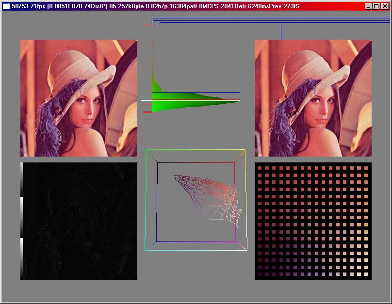
Using this indexed colour idea, we don't get quite far, because we still have to store 8 bits for each pixel when we want to have 256 colours. But now we can use bigger 'cluster' sizes, that means, we can look at a bigger number of pixels together and then do the same as above. But even when just taking 2 coloured pixels, we have 2*3 = 6 dimensional data, which we cannot visualize in a simple way. That program with the screenshots from above then still shows the first 3 dimensions of the codebookvectors in the RGB cube. But we can still take a look at the codebookvectors. As an example we look at a compression using 5x5 pixels as clustersize and 256 codebookvectors. That means that the SOM has now to approximate vectors in a 5*5*3 = 75 dimensional space, instead of the 2 dimensional space showed with the greyscale picture at the start of this article.

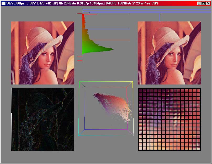
The errors are significantly higher, especially at the edges. The error distribution is also broader. We store 0.91 bits per pixel in this case. This is not optimal, because here we need a lot of space for storing the codebookvectors. Therefore we always have to make a compromise between the size of the codebookvectordata and the size of the indices stored in the file.

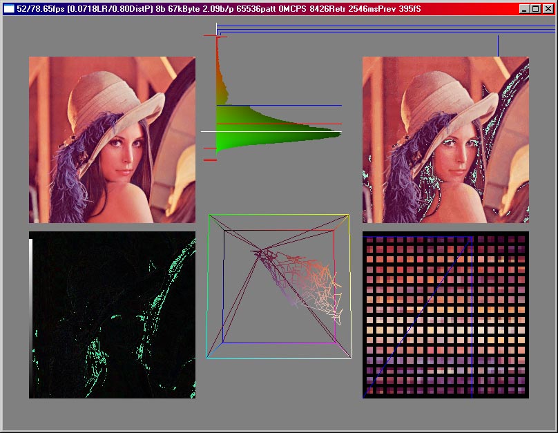
In the following picture, the lena image was compressed using a 2*2 cluster size and 256 codebookvectors. Additionally one codebookvector is marked ( where the blue lines on the codebookvector image cross ) and all the pixels on the decompressed image which belong to that codebookvector are inverted. This way you can see how much of the whole picture is covered by just one codebookvector. Here an index for one of those needs 8 bit, and the codebookvector itself has a size of 3*2*2*8 = 96 bit. Since the lenna picture is 512x512 in size, each codebookvector has an average of 512*512/256 = 1024 pixels being related to it, in this case.

For a table with different clustersizes, different numbers of codebookvector, different topologies look at http://www.lampel.net/johannes/projects/spcc/compress/
'Entropy' and 'sigma' of the picture are just properties of the lena picture. 'Compression quality' tells us if we have used all available clusters for training the SOM or if we have ignored some to speed up the calculation. 1 means that we have taken each pattern available. Then we have the 'number of pattern', which is obviously lower for bigger cluster sizes. The 'topology' tells if we are using a linear or a square SOM. During the training we decrease the distance factor ( and often also the learn rate ) of the SOM, that's 'distance factor decrease'. We stop the iterations once the distance factor has reached 'training end'. 'Retrain' specifies when a pattern should again be given to the SOM for training. A 'Retrain' of 1.5 means that all pattern whose errors are above 1.5 times the average error should be trained again. This might sometimes improve the final results. 'Clustersize' and 'Codebooksize' should be clear. 'bpp' is bits per pixel in the compressed format, including everything, like header of the file, codebookvectors, and index data. 'sigma' is the sigma of the difference between the original picture and the compressed one.

sourcecode:

Using the SOMSim Code, HPTime Code

spcc.cpp ( commandline stuff )
Example.cpp ( windows stuff )
spcc-w.cpp ( windows stuff )
spcc-w.h ( windows stuff )
SOMPCompress.cpp
SOMPCompress.h
IBitStream.cpp
IBitStream.h
OBitStream.cpp
OBitStream.h